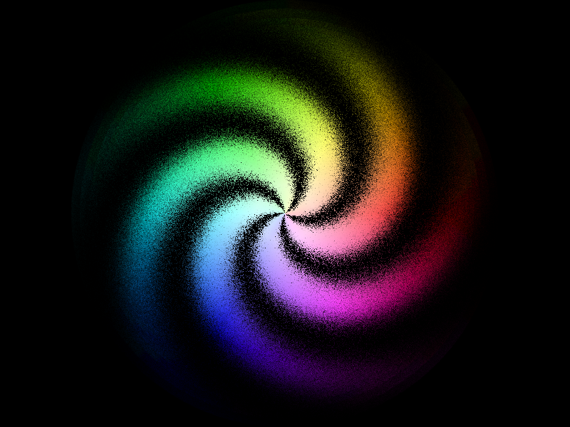
Pixel Visual

The Pixel visual renders individual square-shaped pixels at arbitrary positions. Each pixel has a given size (shared by all vertices in the visual) and a color.

This visual is ideal for raster-style plots or large-scale point clouds, where millions of points can be displayed efficiently with minimal styling.

---

Overview

• Renders square, filled pixels at 3D NDC positions
• Per-vertex: position and color
• Uniform: pixel size (applies to all vertices)
• Supports depth testing for 3D layering
• Efficient for dense, unstructured data

---

When to use

Use the pixel visual when:

• You want to display raw 2D or 3D data points without borders or variable sizing
• You need to visualize millions of points efficiently

---

Attributes

Per-item

Attribute	Type	Description
position	(N, 3) float32	3D positions in NDC
color	(N, 4) uint8	RGBA color per pixel

Per-visual (uniform)

Attribute	Type	Description
size	float	Side length of each pixel in framebuffer pixels

---

Basic usage

visual = app.pixel(position=position, color=color, size=5)

• position: a (N, 3) array in Normalized Device Coordinates (NDC)
• color: a (N, 4) array of uint8 RGBA values
• size: a scalar integer for pixel size in framebuffer pixels

---

Example

import matplotlib.colors as mcolors
import numpy as np

import datoviz as dvz


def generate_data():
    """Return N, positions (N,3) float32, colors (N,4) uint8"""
    # Parameters
    n_arms = 5
    n_particles_per_arm = 200_000
    n_total = n_arms * n_particles_per_arm

    rng = np.random.default_rng(seed=42)

    # Radius from center, with more points toward center
    r = rng.power(2.0, size=n_total)  # values in [0, 1), biased toward 0

    # Angle with swirl per arm and some noise
    base_theta = np.repeat(np.linspace(0, 2 * np.pi, n_arms, endpoint=False), n_particles_per_arm)
    swirl = r * 3  # spiral effect
    noise = rng.normal(scale=0.2, size=n_total)
    theta = base_theta + swirl + noise

    # Convert polar to Cartesian
    x = r * np.cos(theta) * 6.0 / 8.0  # HACK: window aspect ratio
    y = r * np.sin(theta)
    z = np.zeros_like(x)

    positions = np.stack([x, y, z], axis=1).astype(np.float32)

    # Colors based on radius and angle — create a vibrant, cosmic feel
    hue = (theta % (2 * np.pi)) / (2 * np.pi)  # hue from angle
    saturation = np.clip(r * 1.5, 0.2, 1.0)  # more saturated at edges
    value = np.ones_like(hue)

    # Convert HSV to RGB

    rgb = mcolors.hsv_to_rgb(np.stack([hue, saturation, value], axis=1))
    rgb_u8 = (rgb * 255).astype(np.uint8)

    # Alpha: slight fade with radius
    alpha = np.clip(128 * (1.0 - r), 1, 255).astype(np.uint8)
    alpha = (200 * np.exp(-5 * r * r)).astype(np.uint8)

    colors = np.concatenate([rgb_u8, alpha[:, None]], axis=1)

    return n_total, positions, colors


N, position, color = generate_data()

app = dvz.App()
figure = app.figure()
panel = figure.panel()
panzoom = panel.panzoom()

visual = app.pixel(position=position, color=color)
panel.add(visual)

app.run()
app.destroy()

---

Summary

The pixel visual is a fast, lightweight way to display large datasets as colored squares in 2D or 3D space.

• ✔️ Per-point position and color
• ✔️ Efficient rendering of millions of points
• ✔️ Optional depth testing for 3D control
• ❌ No per-point size or shape variation

For symbolic or styled points, see the Point or Marker visuals.