Sphere Visual¶

The Sphere visual renders 3D spheres using GPU impostors — efficient 2D quads that simulate shaded spheres in the fragment shader using raymarching. This allows rendering of thousands of spheres with realistic lighting and minimal geometry overhead.

Overview¶

Each sphere is a screen-aligned quad rendered as a shaded 3D sphere
Positions are in 3D NDC space
Sizes are specified in NDC units or pixels
Lighting parameters are customizable per visual (light support will be improved in a future version)

When to use¶

Use the sphere visual when:

You want efficient rendering of thousands of 3D spheres
You don't need true mesh geometry (no collisions or wireframes)
You want adjustable lighting and shading

Attributes¶

Options¶

Option	Type	Description
`textured`	`bool`	Whether to use a texture for rendering
`lighting`	`bool`	Whether to use lighting
`size_pixels`	`bool`	Whether to specify sphere size in pixels

Per-item¶

Attribute	Type	Description
`position`	`(N, 3) float32`	Center of the sphere (in NDC)
`color`	`(N, 4) uint8`	RGBA color
`size`	`(N,) float32`	Diameter in NDC or pixels

Per-visual (uniform)¶

Attribute	Type	Description
`light_pos`	`vec4`	Light position/direction
`light_color`	`cvec4`	Light color
`material_params`	`vec4`	Material parameters
`shine`	`float`	Shine value
`emit`	`float`	Emission value

Lighting¶

The lighting system is the same as in the Mesh visual.

Example¶

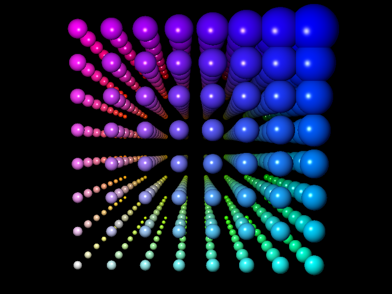
import numpy as np

import datoviz as dvz


def generate_ndc_grid(n):
    lin = np.linspace(-1, 1, n)
    x, y, z = np.meshgrid(lin, lin, lin, indexing='ij')
    positions = np.stack([x, y, z], axis=-1).reshape(-1, 3)

    # Normalize each coordinate to [0, 1] for radius/color mapping
    x_norm = (x + 1) / 2
    y_norm = (y + 1) / 2
    z_norm = (z + 1) / 2

    # Radius increases linearly in all directions (can be tuned)
    size = 0.01 + 0.01 * np.exp(1 * (x_norm + y_norm + z_norm))
    size = size.flatten()

    r = x_norm.flatten()
    g = y_norm.flatten()
    b = z_norm.flatten()
    a = np.ones_like(r)
    rgb = np.stack([r[::-1], g[::-1], b, a], axis=1)
    rgb = (255 * rgb).astype(np.uint8)

    return positions.shape[0], positions, rgb, size


N, position, color, size = generate_ndc_grid(8)

width, height = 800, 600
app = dvz.App()
figure = app.figure()
panel = figure.panel(offset=(0, 0), size=(width, height))
arcball = panel.arcball()

visual = app.sphere(
    position=position,
    color=color,
    size=size,
    lighting=True,
    shine=0.8,
)
panel.add(visual)

app.run()
app.destroy()

Summary¶

The sphere visual provides efficient, realistic rendering of many shaded spheres using fragment-shader raymarching.

✔️ High performance, low geometry cost
✔️ Adjustable lighting and shading
✔️ Ideal for molecular visualization, 3D scatter plots
❌ No physical mesh geometry or edge outlines